Fourier Transform

Basics

The Fourier transform consists in representing an image by its frequential components. You can then process the frequential components image (also called the Fourier image) to perform specific filtering.

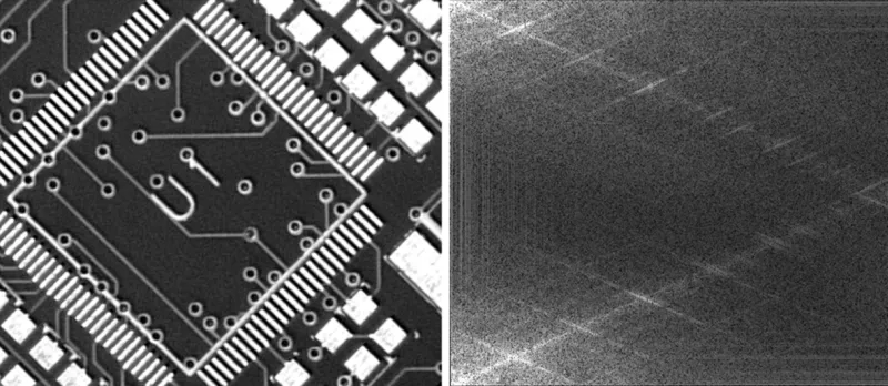
On the left: the image of a PCB, oriented at 45°, and on the right: the corresponding Fourier Image with the frequential structures (scaled for visualization).

Use the EFourierTransformer ^{.NET Python} class to perform the transformation between a spatial and a Fourier image. The Fourier image contains complex numbers and is represented by a floating point image (EFourierImage ^{.NET Python}).

• Use the method EFourierTransformer::DirectTransform ^{.NET Python} to convert a spatial image to an EFourierImage ^{.NET Python}.

• Use the method EFourierTransformer::InverseTransform ^{.NET Python} to convert images the other way around.

Hint

An EFourierImage ^{.NET Python} may contain high values due to the nature of the applied transformation and this may be difficult to display on a screen. For an easier visualization, use EFourierImage::ComputeMagnitude ^{.NET Python} and EFourierImage::ComputePhase ^{.NET Python} to generate an image that can be drawn or saved.

Frequential Format

As the Fourier images contain redundant data, there are different possible representations: Packed and Complex Extended formats. The format is set and used when calling the methods of EFourierTransformer ^{.NET Python}. The format of the EFourierImage ^{.NET Python} can be get and set using EFourierImage::GetFrequentialDomainFormat ^{.NET Python}, but setting a different format does not trigger a conversion.

The Complex Extended Format

The Complex Extended is the simplest of these two formats.

• The only subtlety is that the complex numbers are stored in a floating point array, so the complex extended image is twice larger than the spatial image.

• Each odd column contains the imaginary part of a complex number.

• The following table is an illustration of an image in Complex Extended format, where the complex pixel at row i and column j is: $\(Re (i,j) + i × Im (i,j)\)$

A Fourier Image in the Complex Extended Format

$\(Re(0,0)\)$	$\(Im(0,0)\)$	…	$\(Im(0,w-1)\)$
$\(Re(1,0)\)$	$\(Im(1,0)\)$	…	$\(Im(1,w-1)\)$
…	…	…	…
$\(Re(h-1,0)\)$	$\(Im(h-1,0)\)$	…	$\(Im(h-1,w-1)\)$

The Packed Format

The Packed format is also called Complex Conjugate Symmetrical.

• It takes benefit of the conjugate symmetric properties of the Fourier transform of a real image to reduce the Fourier image size and to be the same as the spatial image size.

• The following table is an illustration of an image in Packed format, where the complex pixel at row i and column j is: $\(Re (i,j) + i \times Im (i,j)\)$

There is a difference between images of odd and even height:

A Fourier Image in Packed Format, Odd Height

\[Re(0,0)\]	\[Re(0,1)\]	\[Im(0,1)\]	…	\[Re(0,(w-1)/2)\]	\[Im(0,(w-1)/2)\]	\[Re(0,w/2)\]
\[Re(1,0)\]	\[Re(1,1)\]	\[Im(1,1)\]	…	\[Re(1,(w-1)/2)\]	\[Im(1,(w-1)/2)\]	\[Re(1,w/2)\]
\[Im(1,0)\]	\[Re(2,1)\]	\[Im(2,1)\]	…	\[Re(2,(w-1)/2)\]	\[Im(2,(w-1)/2)\]	\[Im(1,w/2)\]
…	…	…	…	…	…	…
\[Re(h/2,0)\]	\[Re(h-2,1)\]	\[Im(h-2,1)\]	…	\[Re(h-2,(w-1)/2)\]	\[Im(h-2,(w-1)/2)\]	\[Re(h/2,w/2)\]
\[Im(h/2,0)\]	\[Re(h-1,1)\]	\[Im(h-1,1)\]	…	\[Re(h-1,(w-1)/2)\]	\[Im(h-1,(w-1)/2)\]	\[Im(h/2,w/2)\]

A Fourier Image in Packed Format, Even Height

\[Re(0,0)\]	\[Re(0,1)\]	\[Im(0,1)\]	…	\[Re(0,(w-1)/2)\]	\[Im(0,(w-1)/2)\]	\[Re(0,w/2)\]
\[Re(1,0)\]	\[Re(1,1)\]	\[Im(1,1)\]	…	\[Re(1,(w-1)/2)\]	\[Im(1,(w-1)/2)\]	\[Re(1,w/2)\]
\[Im(1,0)\]	\[Re(2,1)\]	\[Im(2,1)\]	…	\[Re(2,(w-1)/2)\]	\[Im(2,(w-1)/2)\]	\[Im(1,w/2)\]
…	…	…	…	…	…	…
\[Re(h/2-1,0)\]	\[Re(h-3,1)\]	\[Im(h-3,1)\]	…	\[Re(h-3,(w-1)/2)\]	\[Im(h-3,(w-1)/2)\]	\[Re(h/2-1,w/2)\]
\[Im(h/2-1,0)\]	\[Re(h-2,1)\]	\[Im(h-2,1)\]	…	\[Re(h-2,(w-1)/2)\]	\[Im(h-2,(w-1)/2)\]	\[Im(h/2-1,w/2)\]
\[Re(h/2,0)\]	\[Re(h-1,1)\]	\[Im(h-1,1)\]	…	\[Re(h-1,(w-1)/2)\]	\[Im(h-1,(w-1)/2)\]	\[Re(h/2,w/2)\]

• The other coefficients are obtained by using the following properties:

  • For $\(i = 1,…,h-1\)\( and \)\(j = 1,…,w-1\)$:

    • \[Re (i,j) = Re (h-i,w-j)\]
    • \[Im (i,j) = -Im (h-i,w-j)\]

  • For $\(j = 1,…,w-1\)$:

    • \[Re (0,j) = Re (0,w-j)\]
    • \[Im (0,j) = -Im (0,w-j)\]

  • For $\(i = 1,…,h-1\)$:

    • \[Re (i,0) = Re (h-i,0)\]
    • \[Im (i,0) = -Im (h-i,0)\]

See Also

Code Snippets

Easy to understand, ready to copy code snippets.

Fourier Transform

Gabor Filter

Frequency-selective spatial filtering for texture analysis using the Gabor wavelet.

Gabor Filter