EasySegment Supervised¶

To create an EasySegment Supervised tool:

API:
To create an EasySegment Supervised project in Deep Learning Studio:
1. Start Deep Learning Studio.
2. Create a new project and select EasySegment Supervised in the New deep learning project dialog.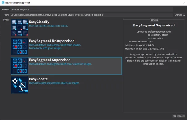
  
  Creating an EasySegment Supervised project.¶

Properties¶

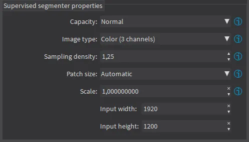
../../../_images/easysegment_5.webp — Tool properties¶

The supervised segmenter tool has 5 parameters:

The Capacity of the neural network (default: Normal) represents the quantity of information it is capable of learning. A larger capacity makes the tool slower.

In the API:
- The capacity is represented by the enumerate type ESupervisedSegmenterCapacity ^.NET ^Python.
- SetCapacity ^.NET ^Python sets the capacity of the tool.
The Image type (default: Monochrome (1 channel)):

In the API:
- To use monochrome (grayscale, 1 channel) images, set SetForceGrayscale ^.NET ^Python to true.
- To use color (3 channels) images, set SetForceGrayscale ^.NET ^Python to false.
The Sampling density (SetSamplingDensity ^.NET ^Python) is the parameter of the sliding window algorithm used to process whole images using patches of size (SetPatchSize ^.NET ^Python).
- It indicates how much overlap there is between the image patches: 100 - (100 / SamplingDensity) (%)
- In practice, the stride between 2 consecutive patches is: PatchSize / SampleDensity (pixels)
The Patch size (SetPatchSize ^.NET ^Python) is the size of the patches processed by the neural network.
- By default, the patch size is determined automatically from the images in the training dataset.
- You can also select the resolution of the patch size from the drop down list.
  
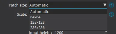
  Patch sizes.¶
Use the Scale (SetScale ^.NET ^Python) to automatically resize your images to a lower resolution and accelerate the processing.

In Deep Learning Studio:
- If the dataset contains images with different resolutions, the Input width and the Input height indicate the range of the resolutions with the given scale.
- If all the images in the dataset have the same resolution, set either the Input width or the Input height to change the scale.

Training¶

To train your tool, see Training a Deep Learning Tool.

Evaluating the Results¶

There are 3 types of metrics for the supervised segmentation tool:
- The pixel-based metrics that quantify the performance of the tool at the pixel level.
- The blob-based metrics that quantify the performance of the tool at the blob level. A blob is a contiguous region of pixels that have the same foreground segmentation label. By definition, there is no background blob.
- The image-based metrics that quantify the performance of the tool at the image level. These metrics are related to the capacity of the tool to correctly detect background images (images with no blobs) and foreground images (images with blobs).
In Deep Learning Studio:
- The metrics are available in the Validation and results tab.
- Most metrics depends on the value of the Classification threshold.
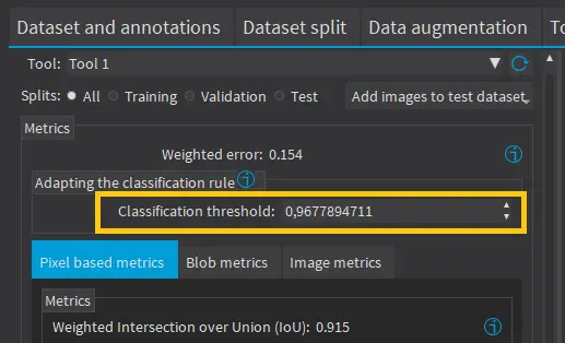
Classification threshold.¶
In the API:
- The metrics are represented by an ESupervisedSegmenterMetrics ^.NET ^Python object.

The Pixel-Based Metrics¶

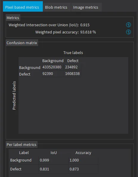
../../../_images/supervised_evaluating_3.webp — Pixel-based metrics¶

The pixel-based metrics are:
- The weighted Intersection over Union (IoU) that is the weighted average of the IoU over all the labels (see per-label metrics).
- The weighted pixel accuracy that is the weighted average of the accuracy over all the labels (see per-label metrics).
- The pixel confusion matrix that shows the number of pixels from a given label that are predicted to belong to another label.
The per label metrics are:
- The Intersection over Union (IoU) that is the ratio of the intersection between the ground truth and the prediction for the label to the union of the ground truth and prediction for the label.
  
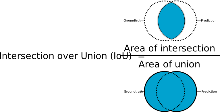
  Intersection over Union
- The accuracy that is the proportion of the pixels of the label that are correctly predicted.

The Blob-Based Metrics¶

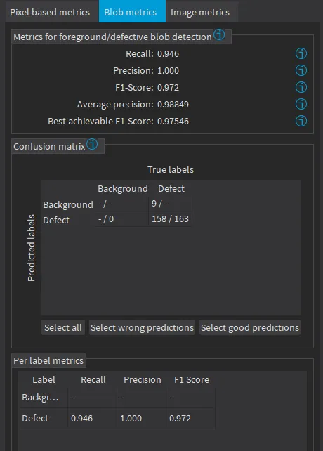
../../../_images/supervised_evaluating_4.webp — Blob-based metrics¶

The metrics related to the correct prediction of blobs are:
- The recall that is the ratio of the correctly predicted blobs to the total number of ground truth blobs.
- The precision that is the ratio of correctly predicted blobs to the total number of predicted blobs.
- The F1-Score that is the harmonic mean of the recall and the precision.
- The average precision that is the average of the precision for different threshold weighted by the recall values.
- The best achievable F1-Score that is the maximum F1-Score achievable by selecting an appropriate threshold.
The confusion matrix:
- It shows the number of blobs of a given true label that are predicted to be of the corresponding predicted label.
- The image list of the Dataset results tab only shows the images containing the blobs corresponding to the selected cells of the matrix.
- Each matrix element shows the number of ground truth blob and the number of corresponding predicted blobs separated by a "/" as a ground truth blob can correspond to one or more blobs in the prediction and inversely.
- A dash (-) indicates that blobs are not defined for this category.
- For example, in the screenshot above, there are:
  - 0 predicted blobs of the label Defect that correspond to the Background (false positive).
  - 9 ground truth blob of the label Defect that does not correspond to any predicted blob (false negative).
  - 163 predicted blobs of the label Defect that correspond to 158 ground truth blob of the same label (true positive).
The metrics for each individual foreground label are:
- Recall
- Precision
- F1-Score

The Image-Based Metrics¶

The metrics related to the correct detection of the class of the images (background / foreground or good / defective in the context of defect detection):
- The image detection accuracy that is the proportion of image correctly predicted to have foreground blobs or not.
- The foreground image detection rate that is the proportion of correctly predicted images with foreground blobs.
- The background image detection rate that is the proportion of correctly predicted images with no foreground blobs.
- The image detection AUC (Area under the ROC Curve, see ROC Curve below).
- The best achievable image detection accuracy that is the maximum image detection accuracy obtained by changing the threshold.
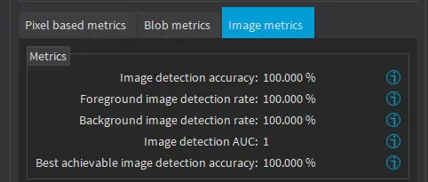
Image-based metrics¶
The confusion matrix:
- It shows the number of images of a given true label that are predicted to be of the corresponding predicted label.
- The image list of the Dataset results tab only shows the images corresponding to the selected cells of the matrix.
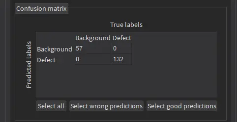
Confusion matrix¶
The 2 available graphics are:
- The ROC curve that plots the true positive rate (foreground image detection rate) versus the false positive rate (1 minus the background image detection rate) for various threshold values.
  
  Click on a point on the plot to set the threshold at the corresponding value.
  
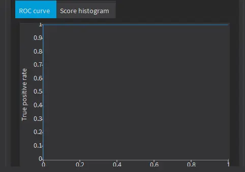
  ROC curve¶
- The score histogram that plots:
  - In green: the cumulative histogram of the scores of the background images.
  - In orange: the cumulative histogram of the scores of the foreground images.
  - The blue line corresponds to the current value of the threshold.
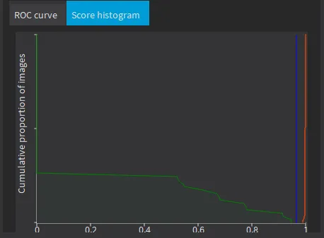
Score histogram¶

Applying the Tool to New Images¶

To get the result, a supervised segmenter follows these steps:

For each pixel, the supervised segmenter tool computes the probabilities that it belongs to each of the segmentation labels.
From these probabilities, it extracts a set of potential foreground blobs (groups of contiguous pixels for which the highest probability corresponds to the same foreground segmentation label).
For each one of these potential foreground blobs:
- It computes a score.
- It removes, from the predicted segmentation map, the blobs with a score that is below or equal to the threshold of the supervised segmenter tool.
The score of an image is the maximum among the scores of the potential foreground blobs.

Note

In the context of defect detection, an image is considered to be without defect when its score is below or equal to the threshold of the supervised segmenter tool.

Deep Learning Studio¶

Include the new images in the test set
1. Add new images to the dataset from the Dataset and annotations tab.
2. In the Validation and results tab, refresh the results
Refreshing or computing new results.¶
Open the Inference tests tab to apply the segmenter to new images and display detailed results for these images.
To visualize the segmentation of an image, check the Predicted segmentation option (CTRL+P) in the Result menu (ALT+R) of the image viewer.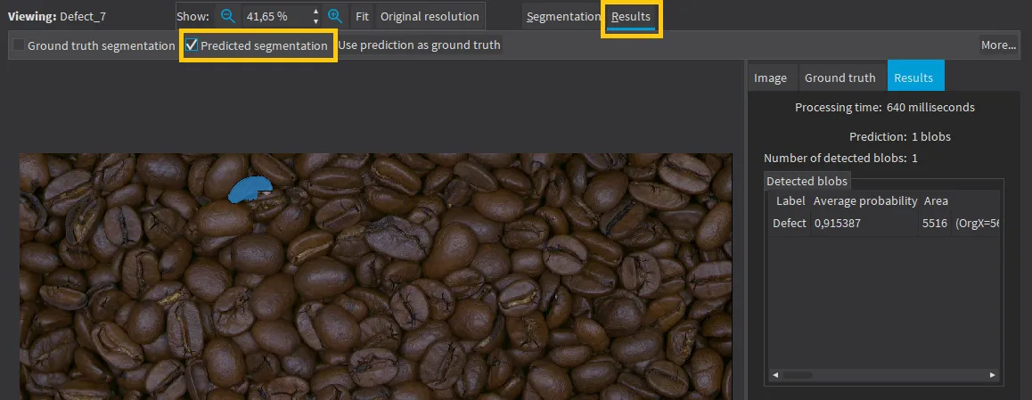

Visualizing the predicted segmentation.
If the image has a ground truth, check the Ground truth segmentation option (CTRL+G) to display it. It appears with a green pattern drawn over it.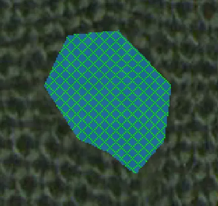

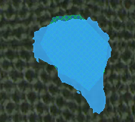
Ground truth (left) and prediction on top of ground truth (right)¶
To accept the whole predicted segmentation as ground truth, click on the Use prediction as ground truth button (CTRL+U).
To accept a single predicted blob as ground truth, right click on the blob and select Accept into ground truth in the menu.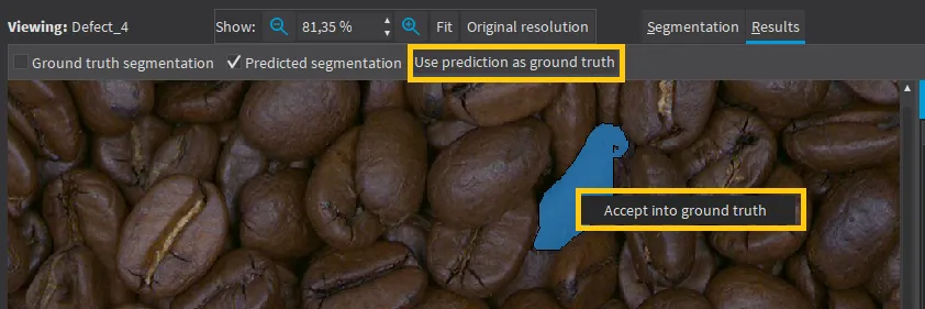

Import prediction into ground truth.
A list of blobs with various characteristics is available in the Results tab of the image viewer.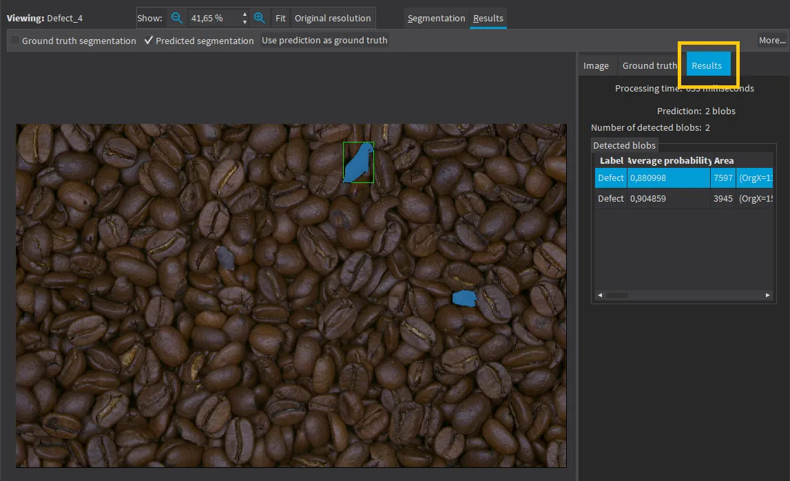

List of predicted blobs.

API¶

To apply the supervised segmenter to an image use ESupervisedSegmenter::Apply ^.NET ^Python. This method returns a ESupervisedSegmenterResult ^.NET ^Python object.
- Use GetProbabilityMap ^.NET ^Python to retrieve the probability map for a given label. The probability map pixels contain the index of the predicted label.
- Use Draw ^.NET ^Python to draw the segmentation with the segmentation label colors of the dataset used for training.
- Use GetBlobs ^.NET ^Python to retrieve the filtered list of blobs.
- Use GetScore ^.NET ^Python to retrieve the score of an image.
- Use GetRegionForLabel ^.NET ^Python to obtain an ERegion object containing the pixels of the specified label.