Easy3DLaserLine - Laser Line Extraction and Calibration

Easy3DLaserLine is used to reconstruct 3D objects from a laser-line triangulation system.

Laser Triangulation

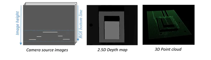
In a laser-line triangulation system, a laser line is projected on the object to measure. A camera is viewing the laser line from a different angle and position. The line deformation observed by the camera contains the shape information of the measured object.

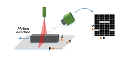
Setup of a laser-line triangulation system.

Scanning the object consists in moving it under the laser line and recording multiple images.

From the scanning you can reconstruct its 3D shape.

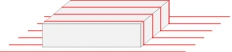
Representation of successive scans of a laser line upon an object.

Occlusions

Using the laser triangulation method, the laser may be unable to reach some parts of the object or the camera may be unable to view them. This is called occlusion.

• On the left illustration, the camera does not see the bottom of the hole, inducing camera occlusion.

• On the right illustration, the laser does not reach the bottom of the hole, inducing laser occlusion.

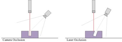
Examples of occlusion that can occur while scanning an object.

Hint

You can limit or avoid occlusions by using advanced scanning methods, for example by using two cameras or two lasers.

Laser Line Acquisition Pipeline

The 3D acquisition pipeline starts with the acquisition of a laser line profile and ends up with the point cloud, mesh or ZMap.

The source material for 3D processing is the depth map, coming from a Coaxlink Quad 3D-LLE or generated from a list of images.

3 types of depth map are available, one for each different pixel coding scheme (8, 16 or 32 bits).

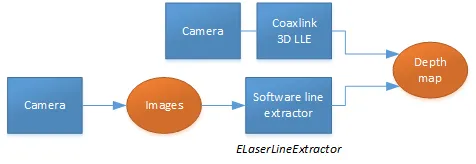
The generation of a depth map, from a hardware or a software source

Some processing methods can use the depth map directly, but most measurement and matching processes need metric, distortion-free representations. Calibration of the laser triangulation setup is therefore required. Calibration is used to turn the depth map into a point cloud or mesh expressed in a metric space that we call “world space”.

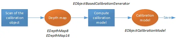
The generation of an object based calibration model, from a scan of the reference object

A point cloud is a list of 3D points, expressed in a world space coordinate system. The point cloud can be projected on a plane, producing a ZMap, which is a convenient and effective representation for 2D processing with a metric scale.

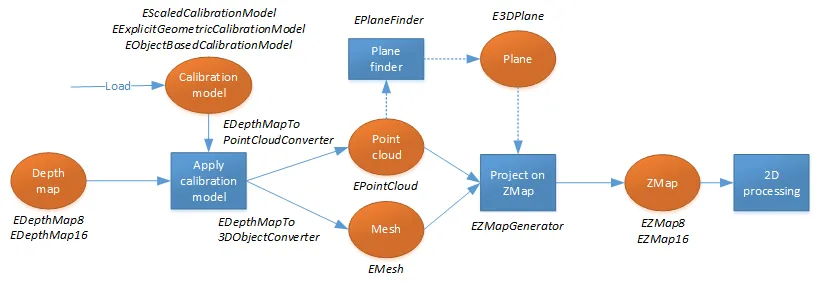
The workflow from the depth map to the ZMap

The following sections describe the classes and methods useful for a 3D workflow. The Measuring a Remote Controller application goes through this processing pipeline.

Laser Line Extraction

A Laser Line Extraction (LLE) algorithm is required to create a depth map from a sequence of profiles of the object captured by the camera sensor.

The objective of an LLE algorithm is to measure the line position along a vertical profile in every column of a sensor frame, within a user-defined region of interest (ROI).

For every step of the object position, the detection analyzes each column of a frame individually and produces a row of output positions, stored as gray values.

The figure below illustrates this process.

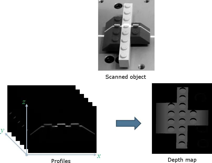
Computation of a depth map using the captured profiles on a scanned object.

The class ELaserLineExtractor ^{.NET Python} provides the laser line extraction functionality.

Use the method ELaserLineExtractor::SetAnalysisMode ^{.NET Python} to select one of the following algorithms to extract the laser line (see below for more details):

• Maximum detection returns the position of the pixel of maximum intensity. It’s the fastest method but it doesn’t support sub-pixel precision.

• Peak detection approach detects local maxima. If several maxima are detected, the one with the highest intensity is returned. The position is returned with sub-pixel precision.

• Center of gravity algorithm is suitable when the laser line is spread over several pixels. The position is returned with sub-pixel precision.

Hint

You can also set a threshold to exclude pixels with low intensity.

The line position returned by the laser line extraction algorithms is relative to the bottom of the region of interest. So, values in the depth map range from 0 (bottom of the ROI) to the height of the ROI.

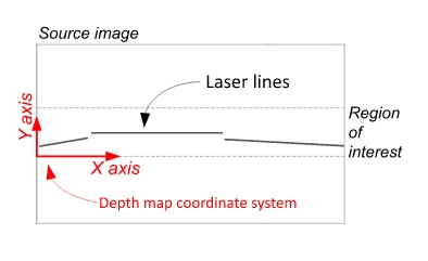
The generated depth map maps its values to the region of interest of the input profiles.

Laser Line Extraction Methods

• Maximum detection

  The maximum detection algorithm analyzes all the pixels in a ROI column to determine the one with the maximum intensity. The figure below shows the laser line position on a given ROI column.

  

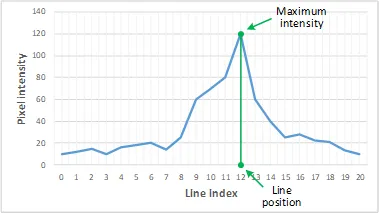
  Maximum detection on a ROI profile

  We also recommend to include in the processing chain:

  • A low-pass filter to reduce the high frequency variations in the image.

  • A threshold to eliminate the background noise from the sensor.

• Peak detection

  The peak detection algorithm relies on a discrete simplification of the first derivative function.

  \(\frac{df}{dx}=f(x+1)-f(x-1)=f'(x)\)

  The \(f'(x)\) outputs the slope of a given \(f(x)\) along the \(x\).

  

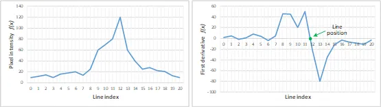
  \(f(x)\) and \(f'(x)\) plots

  We compute the line position by detecting where \(f’(x)\) changes its signal based on the two-point form line equation:

  \(y-y_1=\frac{y_2-y_1}{x_2-x_1}(x-x_1)\)

  where \((x_1, y_1)\) and \((x_2, y_2)\) are two points on the line with \(x_2\ne x_1\), we obtain the following equation for \(y = 0\):

  \(x=\frac{x_1y_2-x_2y_1}{y_2-y_1}\)

• Center of gravity

  The center of gravity (CoG) method uses an algorithm that calculates the center of mass of an image object. Also known as “centroid of plane figures”, the CoG is obtained by the following equations:

  \( \left\{ \begin{aligned} \bar{X} &= \dfrac{\sum ax}{\sum a}\\ \bar{Y} &= \dfrac{\sum ay}{\sum a} \end{aligned} \right. \)

  where \(\overset{—}{X}\) and \(\overset{—}{Y}\) are the coordinates of the CoG and \(a\) is the pixel intensity along the \(x\) and \(y\) axes.

  

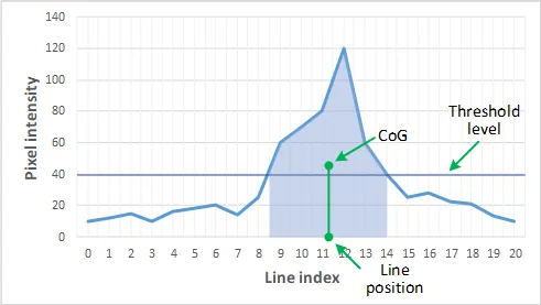
  Center of gravity on a ROI profile

Low-Pass Linear Filter

Optionally, you can apply a low-pass linear filter in front of the line extraction in order to reduce noise and high frequencies in the image.

The low-pass filter applies a convolution operator on a 1 \(\times\) 3 sliding window. The 3 elements of the convolution kernel (A, B and C) are configurable, accepting any positive integer. The figure below illustrates the positioning of the convolution kernel elements within a given ROI.

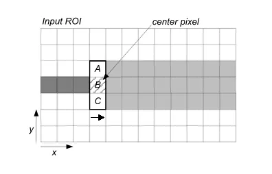
The low-pass linear filter goes through each row and applies a convolution operator on the center pixel.

You can activate the low-pass filter for any of the laser line extraction methods with the method ELaserLineExtractor::SetEnableSmoothing ^{.NET Python}. Parameters A, B and C are set with ELaserLineExtractor::SetSmoothingParameters ^{.NET Python}.

Depth Map Z Resolution

• As explained above, the laser line extraction computes the sub-pixel position of the laser line profile for each column of the region of interest.

  • This position is encoded in a 16-bit depth map (EDepthMap16 ^{.NET Python}).

  • The resolution controls the way the sub-pixel positions are converted to 16-bit fixed point values (that is how many bits are allocated to represent the fractional part of the sub-pixel position).

  • On a EDepthMap16 ^{.NET Python}, use the method EDepthMap16::GetZResolution ^{.NET Python} to retrieve the resolution. It is a floating-point value used to convert the integer pixel value to a real depth value.

• By default, ELaserLineExtractor ^{.NET Python} computes the best resolution depending on the height of the region of interest. The following table lists typical resolution values depending on the height of the processed frame or region of interest.

Frame or ROI height	Bits used for the fractional part	Z resolution
100	8	1/256 = 0.00390625
200	8	1/256 = 0.00390625
400	7	1/128 = 0.0078125
800	6	1/64 = 0.015625
2500	4	1/16 = 0.0625

• Use the optional parameter zResolution of the constructor ELaserLineExtractor::ELaserLineExtractor ^{.NET Python} to fix the Z resolution.

  • If you do not set the parameter zResolution, an algorithm computes the optimal value. Use ELaserLineExtractor::GetDepthMap ^{.NET Python} to query the returned depth map and get the effective resolution.

• If you are using the hardware laser line extraction with the Coaxlink Quad 3D-LLE, the fixed point format is set by the configuration: 8_8 or 11_5 for 8- or 5-bit fractional part.

See also

See Coaxlink’s documentation to LLE processing.

Software vs Hardware Line Extraction

Note

The following information is valid for all tables in this section:

• The region size is given in pixels.

• The extraction speed (fields Max, CoG and Peaks) is given in profiles per second.

Hardware Line Extraction on a Coaxlink

• The Coaxlink Quad 3D-LLE frame grabber features hardware line extraction. The performances are as follows, for all methods - Maximum detection (Max), Center of gravity detection (CoG) and Peak detection (Peaks):

  • 9500 profiles/s for a 2048 \(\times\) 256 or a 4096 \(\times\) 128 region

  • 19000 profiles/s for a 2048 \(\times\) 128 region

  • 38000 profiles/s for a 1024 \(\times\) 128 region

  • 76000 profiles/s for a 1024 \(\times\) 64 region

• As a result, the hardware-based line extraction is \(2\times\) to \(15\times\) faster than the software implementation in eVision running on an Intel Core i7-10850H CPU at 2.70 GHz (see below).

Software Line Extraction on an Intel CPU

The measurement setup is:

• Intel Core i7-10850H CPU at 2.70 GHz

• Generation of 16-bit depth maps

• Methods used: Maximum detection (Max), Center of gravity detection (CoG) and Peak detection (Peaks)

• Using 1 thread, without low pass filter

  Region size	Max	CoG	Peaks
  3072 \(\times\) 512	368	298	248
  3072 \(\times\) 256	752	593	497
  3072 \(\times\) 128	1488	1179	966
  3072 \(\times\) 64	3764	2723	2169
  1024 \(\times\) 512	1142	891	771
  1024 \(\times\) 256	2226	1777	1479
  1024 \(\times\) 128	4266	3324	2752
  1024 \(\times\) 64	11130	8533	6400

• Using 1 thread, with low-pass filter

  Region size	Max	CoG	Peaks
  3072 \(\times\) 512	241	200	183
  3072 \(\times\) 256	468	403	357
  3072 \(\times\) 128	920	790	703
  3072 \(\times\) 64	2169	1765	1610
  1024 \(\times\) 512	707	600	561
  1024 \(\times\) 256	1406	1219	1057
  1024 \(\times\) 128	2723	2370	2048
  1024 \(\times\) 64	6400	5333	4830

• Using 2 threads, without low-pass filter

  Region size	Max	CoG	Peaks
  3072 \(\times\) 512	731	576	474
  3072 \(\times\) 256	1406	1094	941
  3072 \(\times\) 128	2813	2226	1868
  3072 \(\times\) 64	7314	5224	3240
  1024 \(\times\) 512	2000	1718	1446
  1024 \(\times\) 256	4129	3368	2844
  1024 \(\times\) 128	8533	6564	4654
  1024 \(\times\) 64	21333	15058	10666

• Using 4 threads, without low-pass filter

  Region size	Max	CoG	Peaks
  3072 \(\times\) 512	1108	885	703
  3072 \(\times\) 256	2438	1765	1273
  3072 \(\times\) 128	4740	3459	2639
  3072 \(\times\) 64	9481	7757	6564
  1024 \(\times\) 512	3605	2694	2031
  1024 \(\times\) 256	6400	5446	4063
  1024 \(\times\) 128	13473	11636	9846
  1024 \(\times\) 64	36571	19692	19692

Software Line Extraction on a Jetson Nano

• The tables below present benchmarks for software line extraction for various region sizes (in pixels) and configurations. The extraction speed is expressed in profiles per second. The measurement setup is:

  • Jetson Nano (4 available cores). See developer.nvidia.com/embedded/jetson-nano

  • Generation of 16-bit depth maps

  • Methods used: Maximum detection (Max), Center of gravity detection (CoG) and Peak detection (Peaks)

• Using 1 thread, without low pass filter

  Region size	Max	CoG	Peaks
  3072 \(\times\) 512	34	30	30
  3072 \(\times\) 256	126	106	102
  3072 \(\times\) 128	248	210	199
  3072 \(\times\) 64	479	409	374
  1024 \(\times\) 512	110	98	97
  1024 \(\times\) 256	383	321	308
  1024 \(\times\) 128	736	623	587
  1024 \(\times\) 64	1426	1229	1114

• Using 1 thread, with low-pass filter

  Region size	Max	CoG	Peaks
  3072 \(\times\) 512	30	28	27
  3072 \(\times\) 256	112	94	93
  3072 \(\times\) 128	220	188	183
  3072 \(\times\) 64	413	356	333
  1024 \(\times\) 512	90	83	82
  1024 \(\times\) 256	337	285	280
  1024 \(\times\) 128	658	567	543
  1024 \(\times\) 64	1226	1065	987

• Using 2 threads, without low-pass filter

  Region size	Max	CoG	Peaks
  3072 \(\times\) 512	61	56	56
  3072 \(\times\) 256	206	180	181
  3072 \(\times\) 128	423	367	365
  3072 \(\times\) 64	864	740	711
  1024 \(\times\) 512	185	170	168
  1024 \(\times\) 256	596	530	517
  1024 \(\times\) 128	1203	1065	1035
  1024 \(\times\) 64	2403	2106	2000

• Using 4 threads, without low-pass filter

  Region size	Max	CoG	Peaks
  3072 \(\times\) 512	95	91	90
  3072 \(\times\) 256	257	234	240
  3072 \(\times\) 128	515	470	489
  3072 \(\times\) 64	1092	992	1029
  1024 \(\times\) 512	269	260	259
  1024 \(\times\) 256	689	678	675
  1024 \(\times\) 128	1383	1352	1356
  1024 \(\times\) 64	2820	2716	2745

Software Line Extraction on a Jetson AGX Orin

• The tables below present benchmarks for software line extraction for various region sizes (in pixels) and configurations. The extraction speed is expressed in profiles per second. The measurement setup is:

  • Jetson AGX Orin (12 available cores). See www.nvidia.com/en-il/autonomous-machines/embedded-systems/jetson-orin

  • Generation of 16-bit depth maps

  • Methods used: Maximum detection (Max), Center of gravity detection (CoG) and Peak detection (Peaks)

• Using 1 thread, without low pass filter

  Region size	Max	CoG	Peaks
  3072 \(\times\) 512	222	192	181
  3072 \(\times\) 256	449	386	362
  3072 \(\times\) 128	898	766	710
  3072 \(\times\) 64	1796	1521	1391
  1024 \(\times\) 512	671	579	546
  1024 \(\times\) 256	1336	1155	1075
  1024 \(\times\) 128	2680	2301	2106
  1024 \(\times\) 64	5278	4511	4079

• Using 1 thread, with low-pass filter

  Region size	Max	CoG	Peaks
  3072 \(\times\) 512	198	174	164
  3072 \(\times\) 256	401	351	332
  3072 \(\times\) 128	801	697	653
  3072 \(\times\) 64	1592	1380	1261
  1024 \(\times\) 512	600	525	498
  1024 \(\times\) 256	1197	1049	987
  1024 \(\times\) 128	2386	2085	1935
  1024 \(\times\) 64	4697	4096	3696

• Using 2 threads, without low-pass filter

  Region size	Max	CoG	Peaks
  3072 \(\times\) 512	444	382	362
  3072 \(\times\) 256	897	772	723
  3072 \(\times\) 128	1790	1528	1416
  3072 \(\times\) 64	3543	3002	2745
  1024 \(\times\) 512	1338	1158	1088
  1024 \(\times\) 256	2659	2311	2142
  1024 \(\times\) 128	5224	4471	4112
  1024 \(\times\) 64	9941	8533	7529

• Using 4 threads, without low-pass filter

  Region size	Max	CoG	Peaks
  3072 \(\times\) 512	876	763	720
  3072 \(\times\) 256	1790	1530	1436
  3072 \(\times\) 128	3447	3011	2745
  3072 \(\times\) 64	6649	5752	5069
  1024 \(\times\) 512	2687	2321	2178
  1024 \(\times\) 256	5251	4571	4213
  1024 \(\times\) 128	10138	8752	8000
  1024 \(\times\) 64	18618	16516	14422

Calibration

Calibration is used to apply the transformation between a depth map and a point cloud or a mesh.

There are 3 ways to set up this conversion:

• Apply a simple scale on the pixel coordinates of the depth map (EScaleCalibrationModel ^{.NET Python} class)

• Use the explicit geometric model (EExplicitGeometricCalibrationModel ^{.NET Python} class)

• Use the object-based calibration approach (EObjectBasedCalibrationModel ^{.NET Python} class)

These models share the same base class ECalibrationModel ^{.NET Python} and expose the method ECalibrationModel::Apply ^{.NET Python}, which is used to apply the conversion between a depth map pixel and a 3D point. It takes as input the coordinates of one point in a depth map and it returns the coordinates of the corresponding point in the 3D space.

The method ECalibrationModel::Apply ^{.NET Python} is not aware of the possible mirroring of the corresponding depth map and cannot make use of EDepthMap::SetAxisSystemType ^{.NET Python} (see below). If necessary (when the corresponding depth map is vertically mirrored) the \(y\) coordinates should be flipped before calling the Apply method.

• The class EDepthMapToPointCloudConverter ^{.NET Python} generates a point cloud from a depth map, using one of the calibration models.

• The class EDepthMapToMeshConverter ^{.NET Python} generates a mesh from a depth map, using one of the calibration models.

By convention:

• The origin of the referential is the lower-left corner of the depth map.

• The center of the first pixel at the lower-left corner is at \(x = 0.5\) and \(y = 0.5\).

• The center of the pixel at the upper-right corner is at \(x = \text{width} - 0.5\) and \(y = \text{height} - 0.5\), where \(\text{width}\) is the width of the depth map and \(\text{height}\) is its height.

Mirrored Depth Maps

By default, Easy3D considers that the origin of the 3D axis of the depth map is the bottom left of the internal image buffer, and the Y axis is pointing up. This means that the depth map image is not seen as vertically mirrored compared to the real world image of the scanned object.

Nevertheless, depending on your acquisition setup this mirroring can happen (for example if the direction of the scan is inverted).

If this is your case, you can set EDepthMap::SetAxisSystemType ^{.NET Python} to EAxisSystemType_CornerUpperLeft ^{.NET Python}, meaning that the origin of the 3D axis is on the upper left corner and the Y axis is pointing down.

This value changes the behavior of the methods :

• EObjectBasedCalibrationGenerator::Compute ^{.NET Python}

• EDepthMapToPointCloudConverter::Convert ^{.NET Python}

• EDepthMapToMeshConverter::Convert ^{.NET Python}

Scale Calibration

The scale model (EScaleCalibrationModel ^{.NET Python}) only applies a simple factor on the X, Y and Z axis. These factors are the only parameters of EScaleCalibrationModel ^{.NET Python}.

For depth maps coming from laser triangulation setup, this transformation does not produce corrected, metric points. It’s main use is to display depth maps as 3D data with the E3DViewer ^{.NET Python} class.

Explicit Geometric Calibration

The explicit geometric model (EExplicitGeometricCalibrationModel ^{.NET Python}) defines a simple and ideal laser triangulation setup. The explicit calibration makes some strong assumptions on the setup geometry and can only be used when a minimum set of parameters are known:

• The angles of the camera and the laser plane, in the counter clockwise direction. The camera angle must be positive.

• The height of the camera above the scanned object.

• The field of view of the camera defined by the sensor size (mm) and the optical focal length (mm).

• The physical distance between two line scans of the depth map (depends on acquisition rate and motion speed).

• The size of the image and the ROI origin used in laser line extraction (between the top (0) and the bottom (height) of the image).

Hint

Use the “Easy3D_Setup_Configuration.xlsx” spreadsheet to compute and check your setup configuration and parameters.

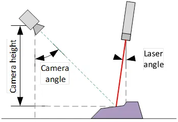
Explicit calibration setup with camera angle, laser angle and camera height

The setup of an explicit geometric calibration uses the constructor of the EExplicitGeometricCalibrationModel ^{.NET Python} class.

Object-Based Calibration

Object-based calibration gives real world, metric, coordinates from an arbitrary laser triangulation setup. From the scan of a reference object, the calibration process tries to calculate all the parameters required for the transformation to the world space (position and attributes of the camera, position of the laser plane, relative motion of the object, optical distortion…).

Object-Based Calibration Guidelines

Easy3D calibration is a powerful process that uses a single scan of a calibration object to calibrate a laser triangulation setup.

1. The calibration process generates a calibration model.

2. Easy3D uses this calibration model to transform the laser profile scans (or depth maps) into metric, distortion free point clouds.

• The calibration model includes all the geometric parameters required for this transformation:

  • The relative position of the laser and the camera.

  • The projection and the distortion model of the camera.

  • The relative motion of the object.

This document explains all the steps involved in the calibration process, from the design of the calibration object to the eVision API.

The Calibration Object

The general principle of Easy3D calibration is to match a scan of a known calibration object to its true geometric dimensions.

The Truncated Double Pyramid

• The dimensions of the “double truncated pyramid” calibration object the X-, Y- and Z-axes are named A, B and C respectively.

• The design of the double truncated pyramid must follow the ratios given in the illustration below.

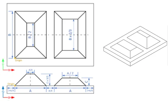
The “double truncated pyramid” calibration model (recommended)

• For example, the provided CAD files of the calibration object use A = 4 cm, B = 6 cm and C = 1 cm. The Calibration Object Size, required for the calibration process, are the values A, B and C.

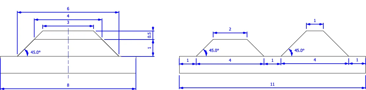
The “double truncated pyramid” calibration model with A = 4, B = 6 and C = 1

Building a Calibration Object

Overall Dimensions

• Manufacture a calibration object that fits the working area of the project.

• For example, if the project targets the inspection of a PCB (a printed circuit board as illustrated), design your calibration object with:

  1. The dimension A or B (it does not matter) similar to the width of the PCB.

  2. The height (C) of only several millimeters.

Hint

This is not a strict requirement, if the scanned object is slightly larger or smaller than the calibration object, the calibration process is still valid.

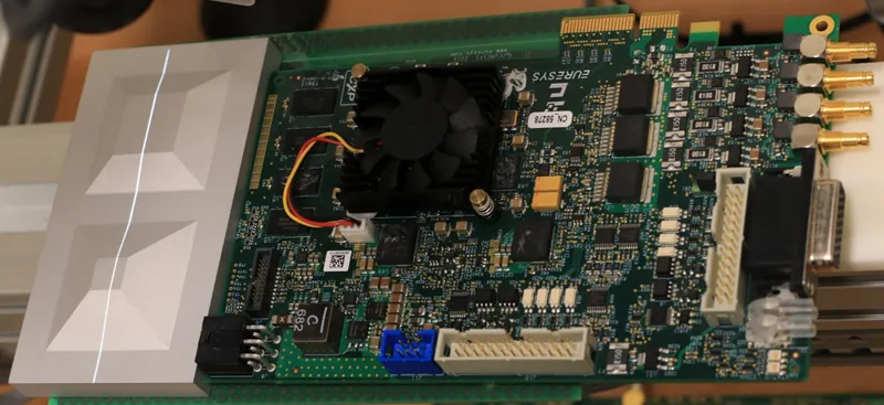
A PCB scanning setup with the associated calibration object. The calibration object dimensions (A, B and C) match the width and the height of the PCB

Hint

There is no constraint on the orientation of the calibration object during the scan:

• The X-axis can be aligned with the motion direction or with the laser line.

• After the calibration process, the origin and axes of the 3D calibrated point cloud follow the conventions of the reference design.

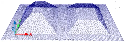
A calibrated point cloud with the origin and the axis of the coordinates system. The 3D origin is located at the external corner of the higher pyramid

Precision and Tolerance

The relevant dimensions of the calibration object are the width, the length and the height of the pyramids (called A, B and C in the illustrations).

• The relative dimensions to A, B and C (B/2, A/4…) are important and you must execute them with the same precision.

• The dimensional tolerances are related to the overall expected precision. If you want to achieve measurements on the point cloud with a precision of 0.01 mm, the manufacturing of the calibration object must have the same precision.

• These tolerances only apply to the pyramids geometry, the calibration process does not use the dimensions of the support.

• The planar surfaces must be flat between 2 parallel planes separated by the target tolerance, as illustrated.

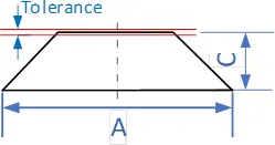
The tolerance of the pyramids sides is defined as the smallest distance between two parallel planes that contain the entire surface

Material and Surface Finishing

Hint

The goal is to obtain the laser profile as thinnest as possible over the whole object surface with the largest reflected energy.

The build material and the surface finishing are also important and must have:

• A good reflectance, with diffuse reflection (no specular reflections).

• No transmission and limited diffusion inside the material.

Hint

You can obtain a good surface finishing using aluminum material and blasting. Blasting gives the surfaces a satin gray finish.

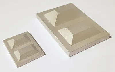
2 aluminum machined calibration objects with a micro-abrasive blasting surface treatment

3D CAD Models

The calibration object models are available in various 3D CAD formats like STEP, OBJ and STL.

Download these files from the download area in the Additional Resources section (www.euresys.com/Support).

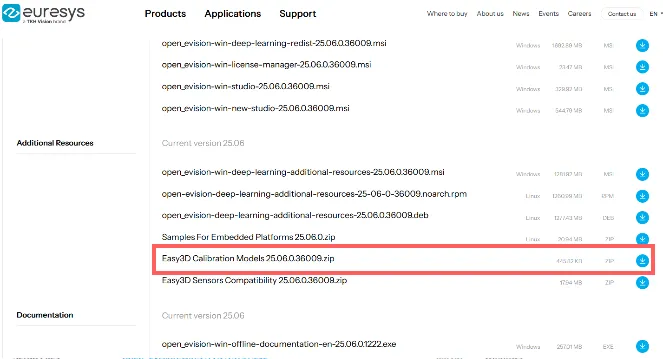
Download the calibration object models

Scanning the Calibration Object

• The scan of the calibration object produces a depth map.

• To ensure a correct detection of the calibration object and a precise calibration model, you must fulfill the following criteria:

  • All faces of the calibration object must be visible on the depth map (this affects the orientation of both the camera and the laser).

  • No other object can be higher than the calibration object in the depth map.

  • The depth map must have at least 200 \(\times\) 200 pixels.

  • The calibration object must cover at least 50% of the defined pixels of the depth map.

• Examples of bad scans:

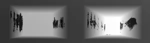
Missing pixels on the side faces

Not enough lines

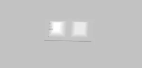
The calibration object is too small on the depth map

Using the calibration with eVision

• The class EObjectBasedCalibrationModel ^{.NET Python} is the container for the object based calibration model.

• The class EObjectBasedCalibrationGenerator ^{.NET Python} performs the computation of such a model using an EDepthMap8 ^{.NET Python}/EDepthMap16 ^{.NET Python}/EDepthMap32f ^{.NET Python} as input.

See also

• Code snippets

• C++ sample